
O1.M2.01. Tools for visualizing the urban geography of economic growth Case study: The urban geography of economic and social growth in Romania 2010-2020
Free
About this course
Session 1: The urban geography of economic and social growth in Romania 2010-2020
Teaching method: lecture
Duration: 120 min
Content:
In which categories do the cities from Romania fall from the perspective of the economic and social changes through which they underwent in the last decade? Does this typology indicate a change in the patterns of economic and social geography of Romania? Can we delignate the trajectory of specific cities in the new economic and social landscape? Take the case of Jimbolia: where does it stand? Is Jimbolia a growing, static or a shrinking city? What kind of resources and capabilities does it uses in the changing landscape of capital investments?
Despite population loss emerging as a general trend for urban settlements in Europe, more recently a reverse trend of regrowth has become evident in certain cities (Kabisch, Haase, and Haase 2010). The existing literature regarding regrowth follows two distinct paths. The first one is engaging with the idea of reurbanization and argues for the increase of population density within the city (Broitman and Koomen 2020; Kabisch et al. 2010; Wolff et al. 2017), while examining the impact on the built-up area and green spaces (Wolff et al. 2017). The second narrative distances itself from the argument for densification and the concept of reurbanization, by examining the current dynamic from the framework of extended urbanization. Keil (2018) argues that what we witness is a new process, one which differs qualitatively from reurbanization. The focal point in his analysis is that of suburbanism, which is seen by the first set of positions rather as a driving force for population loss. On the contrary, the second set of positions, along Keil (2018), considers the contemporary practices of urban peripheralization to be structurally different and more complex than what are traditionally thought of as suburbs, naming the phenomenon post-suburbanism. To be more precise, the problem of regrowth is not one strictly related to the urban core, but it has more to do with a process of complexification of the landscape and social relations existing at the periphery of the city. Starting from this point of tension between the two bodies of literature, the present paper reflects on the ongoing dynamic of population regrowth and certain cities of Romania. Special attention is paid in this regard to peri-urban localities and their transformation in the last decade, as they are specific local examples, closely related to what Keil (2018) envisaged as post-suburbia.
We argue that we witness in Romania post-shrinkage growth: while the urban core is contracting demographically, the suburbs are increasing and densifying. Eastern Europe became the focus of research on urban shrinkage in the 1990s, but the focus of the literature was on post-socialist transformation. The process of urban contraction is generally analysed from a rigorous demographic perspective to address depopulation and recent demographic changes (Bănică, Istrate, and Muntele 2017; Eva, Cehan, and Lazăr 2021), or from the broader framework of deindustrialization (Popescu 2014). Moreover, the current literature follows the larger European academic trend of case studies on shrinking identities and trajectories, through in-depth studies of Timișoara (Lucheș, Nadolu, and Dincă 2011; Rink et al. 2014), Bucharest (Ianoş et al. 2016) or the mining cities of Valea Jiului (Constantinescu 2012). However, recent scholarship emphasized upon the multi-causality of shrinkage (Haase et al. 2016; Martinez-Fernandez, Audirac, et al. 2012; Wolff and Wiechmann 2018) and how localities respond to it (Pallagst et al. 2021). This paper aims to move away from the generic postsocialist framework and deindustrialization to build a typology of urban shrinkage in Romania by including variables that encompass the multiple dimensions of the process: demographic, floor space, economic, human development, urban governance, city expenditure and the environmental situation.
The existing debates revolve around concepts such as reurbanization (Kabisch, Haase, and Haase 2010; Wolff et al. 2017) on the one hand, and extended urbanization (Keil 2018) and post-suburbia (Charmes and Keil 2015), on the other hand. Reurbanization is of concern for urban scholars who study suburbanization as concomitant with urban shrinkage. For much of this literature, the urban life cycle model of van den Berg, Drewett and Klaassen (2013) supports the claim that these two tendencies are distinct sequences in a cyclic model of growth and decline. Another central aspect to reurbanization is the problem of densification, which is seen as happening either in the urban core (Broitman and Koomen 2020) or in certain places within the city. However, in this framework, while temporarily simultaneous, suburbanization and shrinkage are perceived as an opposing spatial trend: core shrinkage fades away as population returns in the core from suburbia (Kabisch, Haase, and Haase 2010).
Extended urbanization and post-suburbia are, on the other hand, key concepts in Roger Keil’s analysis of contemporary urbanization (Charmes and Keil 2015; Keil 2017). Post-suburbanism refers to the structural changes which alter the internal organization of the suburbs. This is the outcome of the process of extended urbanization which re-shapes the peripheries of the cities. Our paper follows this second corpus of literature, and we avoid a simple opposition between shrinking and growth and follow a more complex typology of urban dynamic. More specifically, we interpret the shrinkage of the urban cores as a process which pertains to extended urbanization, without having some strong assumptions about urban life cycles.
During this class we make four inter-related points. First, we argue that one form of post-shrinkage growth is that of the larger urban agglomerations that went through an urban core shrinkage, while their periurban experienced population growth. Second, we show that another form of post-shrinkage growth is that of mid urban agglomerations that experience economic growth and inner densification, while they were demographically shrinking both in the urban core and in their periurban area. Third, we point towards several type of post-shrinkage growth, where economic densification and growth was primarily located in the periurban area, while the core experienced both demographic and economic contraction. Forth, we demonstrate that, indeed, in Romania, some cities experience shrinkage in its classical form, that is both demographic and economic, simultaneously in its core and in their periurban area.
Methodology
To classify the Romanian cities, we use three steps.
- The selection of the variables used in the analysis. First, we select demographic (age composition), economic (turnover, employment, sector) and social variables (education) that describe different aspects of cities’ dynamic, keeping in mind the particularities of the geography of growth in last decade in Romania. There are two major classes of variables that we selected in our analysis: on the one hand, we used variables that describe the changes of the labor force and more broadly the improvement of the wellbeing of the population, and on the other hand we used variables that capture the changes in the distribution of the capital at local level.
- Data reduction using principal components. Second, we summarize the datasets using principal component analysis, a method that reduces a large set of attributes to a smaller, more manageable one, synthesizing the variability of the initial set into its principal axes of variation (Shlens, 2014). The reduced data are related to the income of the workforce, the sectorial structure of the labor force, its wellbeing (public spending, residential space, green space, air quality) and data that quantifies spill-over effects (human development, human capital, natural growth, age structure, and volume change).
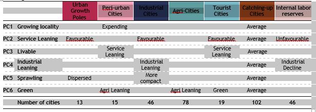
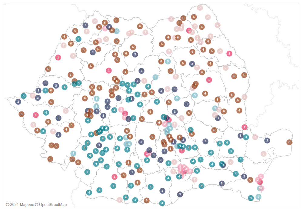
3. Clustering algorithm based on the principal components. Third, we classify the Romanian cities using a k-means algorithm (Hartigan & Wong, 1979) based on the principal components that summarized the initial set of data in the previous step. We obtained a classification of the Romanian cities in seven classes. The results are shown in Table 1.
Seven major types of cities
Urban Growth Poles are grouping together the cities that score high on the sprawling and livable component (both being negatively corelated with the rest of the components). On average, these group of cities (Brașov, Bucharest, Cluj-Napoca, Constanta, Craiova, Galați, Iași, Oradea, Pitești, Ploiești, Sibiu, Suceava, Timișoara) had an increase in population the peri-urban area of 32% and an increase of the floor space with 40%. On average, the population in the urban core contracted by 3%, even if the floor space in the core area expended with 40% since 2009 and with 90% since 1990. These cities have, on average, the biggest human development index and the highest attainment rate of the secondary school diploma (the exam is called in “baccalaureate” as in the French educational system). These cities are the most populous from Romania, visible in the high average of citizen for each city hall employee and have some of the best public infrastructure networks, visible in the high degree of the population coverage of the public transportation system. The number of new-borns in the peri-urban area is the smallest compared with all the other groups of cities since the ration of urban core population to the peri-urban area is the smallest.
More precisely, the peri-urban population represent 20% of the total sum from the urban core and peri-urban area – the share being 32% across the urban network from Romania. Nonetheless, these are the cities that have expanded their urban footprint the most in the last 10 year, generating urban sprawl beyond their administrative boundaries.
Peri-urban Cities are the receivers of the sprawl pressures from the urban poles of larger cities. Fifteen cities have been classified as peri-urban cities, even though, in terms of geographical position there are 62 peri-urban cities. The difference come from the specific traits of being a major buffer for the expansion of the urban pole from the nearby. Bucharest has created a huge stress on its neighboring cities (Bragadiru, Buftea, Chitila, Năvodari, Otopeni, Ovidiu, Pantelimon, Popești-Leordeni, Voluntari), but is not the only one. Brașov, Ploiești, Pitești, Constanta are surrounded by quite a large network of towns that grew both in population and in their urban footprint in the last decade. All the urban growth poles have generated sprawl in their periurban area, yet many of surrounded localities are communes. Most notably are Cluj-Napoca (with the spectacular population burst of Floresti, Apahida and Baciu), Timișoara (with explosive growth of Dumbravița, Giroc and Moșnișa Nouă), Iași (with the expansion of Valea Lupului, Miroslava and Rediu). Similar processes of peri-urban growth by more than 60% of the population in the neighboring commune happened near Brașov (Sânpetru) Craiova (Malu Mare and Carcea), Oradea (Paleu and Sântadrei) or Sibiu (Selimbăr). The peri-urban cities had on average a 36% boom in population and 72% increase in floor space. The local human development index is the largest among all the groups of cities, yet they have the lowest attainment rate for secondary school diploma (36%). This suggest that the peri-urban cities are places of major social inequalities among the households and that they are affected by a selective filtering of the students: the children of the well-off parents are commuting to the better schools. The peri-urban cities are not only site of population growth, but also expansion sites for business (visible in the high number of businesses per capita), yet peri-urban cities are not the only site of the economic sprawl, but the whole peri-urban area of the growth poles (visible in the share of per-urban private companies). A particular case is Baia-Mare, a county capital with an industrial profile and not an urban growth pole, yet it neighbors an expanding per-urban city Tăuți-Măgheruș, where most of the peri-urban growth of Baia Mare was absorbed.
Industrial Cities have experienced a contraction of the population in the urban core, on average by 4%, they have witnessed a moderate growth in population and business within their peri-urban area, but have avoided urban sprawl. They host large companies, with many employees, generating at city level a significant gross local income per capita. On average one third of the of the employees are working in industry (i.e. Alba Iulia, Arad, Baia Mare, Bistrița, Brăila, Buzău, Focșani, Miercurea Ciuc, Odorheiu Secuiesc, Piatra Neamț, Satu Mare, Târgu Mureș) and, on average, these cities have personal incomes per capita above the national level. Both the human development index and the attainment rate of secondary school diploma is quite high. To sum up, this class of cities scores high on the industrial leaning and the livability components simultaneously. Nonetheless, there are important variation in this class of cities in term of size and rate of growth, hence a more detailed analysis is needed here.
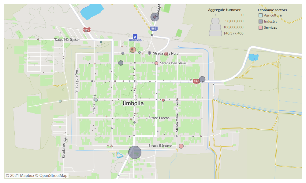
Agri-Cities have a higher number of employees in agriculture compared with the national average. Nonetheless, the average percentage is quite small: 1,6%. However, these cities have, on average, the worst quality of the air and quite modest green spaces per capita. The component that we called ‘green’ captures a geographical correlation between three relatively independent variables: employment in agriculture, green areas in hectares and air quality. Still, it groups together the cities that have large agricultural lands at their disposal. The specificity of highly mechanized agriculture is that it employs quite a small workforce. Most of these cities are placed in the Romanian Plain in the South of the country and in the Transylvanian Plain, the area with the worst? air in Romania. There are 78 cities grouped in this cluster and the internal variability of the cluster is quite large, suggesting the need to further differentiate within this group. Jimbolia is one of those cities. The specificity of Jimbolia is that, economically, the urban core is growing. In Jimbolia there are three types of economic expansion: in terms of employees (2020 compared with 2003), aggregate turnover grew (2018 compared with 2011), and personal income tax, that is wages (2009 compared with 2019). Approximatively two thousand people are employed in manufacturing. However, most of its growth is linked to the new cable factory and the fact that is a direct foreign investment. Nonetheless, compared with the other cities in Romania is endowed with quite a large agricultural land and a high efficiency in terms of turnover per employee. Despite just 68 employees in agriculture, the aggregate turnover is 8,5 million euro and 123 thousand euro per employee. Compared with similar the 38 thousand euro per employee, the average in the cluster, Jimbolia stands out in terms of agri-business.
Tourist Cities. They also score high on the ‘green’ component, but there are the cities which on average have the best air quality and most green spaces per capita. One in ten employees are working in commercial services, and more specifically, they are working in the hospitality industry. These are places with important social inequalities revealed by an above the average human development index and a small attainment rate of secondary school diplomas. Many of these cities are surrounded by rural localities in their peri-urban area, which explain the higher natality in the peri-urban. Nonetheless, these cities were quite successful in attracting EU Funds and were able to invest the most in expanding their local infrastructure and amenities.
Catching-up Cities is a generic catch all cluster that groups together cities that do not have any specific traits given our initial selection of variable driven by the interest to differentiate the cities based on the composition of the labor force. It groups 102 cities and, therefore, a more detailed analysis is needed to further describe these and to differentiate among them.
Cities with internal labor reserves are those who score, on average, low on the livability index and industrial leaning components. The gross local income per capita is the smallest from all the clusters. These cities remain rather static in terms of population both in the urban core and the peri-urban area, yet the children dependency rate suggest a young population overall. The cities tend to be surrounded by rural peri-urban localities, that act as a continuous economic hinterland dominated by agrarian activities There are rather few employees in the industrial sector and commercial services. There are 46 cities in this group and a finer grain drill down is needed to further describe this cluster.
Discussion: the geography of urban growth
This typology of the urban localities from Romania points to a new geography of economic and social growth in Romania. The significance of the typology must be put in a larger picture that takes into account transformation at the national and continental scales. Romania economy grew since 2011 with an annual average of 3.9%, above the Central and Eastern European average of 3.2% and significantly more above the European Union average of 1.4%. Romania’s economy recovered from the Financial Global Crisis of 2008 only in 2011, while the Eastern Europe, along with the rest of European Union, recorded signs of recovery in 2010, (data.WorldBank.org NY.GDP.MKTP.KD.ZG). Romania had a contraction of 5.5% in 2009 and 3.9% in 2011, which is not a surprise given the important role played by exports and the complex interwoven character of the national economy to the global markets.
Volume of exports. In 2019 Romanian’s GDP was $250.1B (data.WorldBank.org NY.GDP.MKTP.CD) and its exports, both of products and services, amounted, in current USD, to 39,6% of its GDP, with a peak in 2017 of 43.2% (CEPII International Trade BACI HS1996-2019 & UN ComTrade Services EB02). In 2008, just before the Economic Crises the total exports represented 34.6% of the GDP, with a major contraction in 2009 of 18%. However, since 2011 Romanian exports increased annually with 4.8%, and the value of the product exports increased the most. By 2019 the value of the product exports was 80% of the total value exported, and only 20% the services. In 2008 the balance was still tipping toward a 67% for product exports, yet the services were one third of the total (CEPII International Trade BACI HS1996-2019 & UN ComTrade Services EB02).
Foreign direct investments. Romania product exports are heavily driven by foreign direct investments: 83% of the value of products exported in 2019 was of companies with foreign capital (INS Tempo EXP101R). This structure of the exports was reflected in employment growth. In Romania, in 2019, 26% of the employees in the private sector were working for a company with full foreign capital (INS Tempo FOM104B); these companies produce 52% of the total aggregate turnover and 45% of the total gross value added (Cristescu, 2020:3). Romania is far from unique in terms of its economic model (Drahokoupil & Fabo, 2020; Nölke & Vliegenthart, 2009). In fact, this type of development is specific for Eastern Europe, yet Romania does excel (Ban, 2019) and this has important geographical consequences.
Urban economic growth. The aggregated revenues of the companies in Romania (the sum of all the revenues) increased by 59.9% between 2008 and 2019, and by 52.4% compared to 2011 (). Between 2011 and 2018, Bucharest grew only by 6.5%, nonetheless, it concentrates 28.1% of the national turnover. The modest growth of the capital is due to a change in the economic geography of Romania: the cities with more than 110T inhabitants became increasingly important, their economy grew by nearly one half (48%) in less than a decade (). In addition, the cities with more than 110T inhabitants, except for the capital, collectively produced 59.6% of all the company’s revenue. The economy of the towns with less than 110T stagnated and concentrated in 2018 only 17% of Romania’s turnover ().
Peri-urban growth. The localities from the peri-urban area surrounding the cities with more than 110T inhabitants had a 65% spectacular growth in aggregate turnover. The companies’ revenue of the 171 communes from the peri-urban area of the cities with more than 110 T inhabitants was the same as of the rest of the 2719 communes in the country – namely 8%. In addition, the localities in first ring around the cities with more than 110T inhabitants registered the largest increase in the number of employees. In these peri-urban areas the percentage of employees increased by 76% between 2011 and 2018. Localities in the second ring around cities registered an increase of 39% of employees ().
The pillars of the economic growth. The economic growth of the cities must be placed in a bigger economic landscape: 45% of the labor force in manufacturing were working in a company owned by foreign capital and these companies were producing 68% of the sector’s aggregate revenue (Cristescu, 2020:3). After 2008, the economic recovery was predicated on two pillars: manufacturing outsourcing (MO) and information technology outsourcing (ITO). First, the manufacturing sector since 2011 had the biggest impact on the GDP growth – an annual average of 24.0% of the GDP growth (INS “Comunicat evoluția PIB” Series). Second, Romania had a huge surge in the ITC sector in the last decade, the sector being the second largest contributor to GDP growth since 2011 – with 16% (INS ‘Comunicat evoluția PIB’ Series). After 2008 Romania economy have been restructuring in important ways and these new developments had major spatial consequences given the dynamic of investments at local level. The cities themselves became important economic engines.
Global outsourcing. After the financial crisis, globalization processes have intensified, and as such, global organizations relocated their secondary processes to new spaces specialized in operations. The new wave of outsourcing is not only focused on industrialized labor, but also on finding skilled and highly skilled labor pools (Peck, 2018). Most of the processes that are being externalized are Business Process Outsourcing (BPO) and Information Technology Outsourcing (ITO) (Oshri, Kotlarsky, & Willcocks, 2015). Even if it is work performed by white collars, the outsourced jobs have a high level of routine and standardization. However, there are some notable exceptions, with the outsourcing of information technology there are outsourced also some key R&D operations (Santangelo, Meyer, & Jindra, 2016). At European level, Central and Eastern Europe has capitalized most of the outsourcing both of manufacturing and business processes from the companies located in Western Europe (Ban, 2019; Drahokoupil & Fabo, 2020). As mentioned before, Romania has benefited from this new trend and it became a destination for foreign capital once again after 2011. However, this time it became a destination both for manufacturing outsourcing and for services outsourcing.
Manufacturing outsourcing. In Romania, after 2011, the aggregated turnover of the industrial sector increased with 56%, while at European level it increased with 16% (EUROSTAT nama_10_gdp). In addition, the added value of the industrial sector increased with 47% in Romania, while at European level it had a modest increase of 6% (EUROSTAT nama_10_gdp). The total number of employees in the industrial sector in Romania is below the 2008 peak value (88%); nonetheless, industrial labor productivity in manufacturing increased from 2008 to 2018 with 73% (INS Tempo IND105E). In terms of employees, most of the industrial production in Romania is in the cities with more than 110T inhabitants (42,8%). Also, an important part of the industrial production is in smaller cities scattered especially in Transylvania and on the corridor of Bucharest, Ploiesti, Pitesti, Brasov. The biggest growth in industrial jobs was in the last ten years in the peri-urban areas of the cities and in villages. That is because most of the new industrial parks were greenfield projects, most of them located in Transylvania. However, just 8.5% of the industrial activities are in rural areas which are not seated in the peri-urban area of a city.
Services outsourcing. In 2020, from the total of 219.5 T of people employed in IT&C in Romania 71.2% are based in Bucharest, Cluj, Timiș and Iași counties (INS Tempo FOM105F), and most of them are working in the county seats cities. In addition, from the 100.7 T of employed persons in financial and insurance services in Romania, 58.7% are working in the same counties, and more precisely in four major cities: Bucharest, Cluj-Napoca, Timișoara and Iași (INS Tempo FOM105F). The average monthly net wage in IT&C in dec. 2020 was 1706 € and in the finance and insurance sector it was 1494 €. The national average across industries was 743 € (INS Tempo FOM106D). In Cluj county the average in IT&C net wage was with 26% more than the national average (INS Tempo FOM106E). Also, in Cluj-Napoca, in July 2020 more the one in ten employees was working in IT and, more generally, one in five employees was working in the outsourced service sector (Petrovici, Săcuiu, & Petrovici, 2020). On average, in 2019, at national level the net wage was 60.2% bigger in a foreign company as opposed to a private local company (INS Tempo FOM106B) and most of the well-paid outsources service jobs were the prerogative of the four cities. The dynamic can be synthetically captured by a staggering figure: 57% from the total taxes on wages came in 2019 from the four cities.
Jimbolia has also benefited from direct investments in the last decade, changing the trajectory of the city. In 2020 in the city 90% of the aggregate turnover of the locality in manufacturing was generated by foreign companies. Moreover, half of the aggregate turnover of the locality was produced by the manufacturing foreign companies. In addition, a quarter of the aggregate turnover of the locality in service is generated by foreign companies. However, most of it is produced by companies in commerce. Nonetheless, there are foreign companies in business consultancy located in Jimbolia.
Conclusion
A historical note must be made here: the Romanian urban network developed after 1947, up until then 78% of the population was rural (Rotariu, Dumănescu, & Hărăguş, 2017). The urban network was not really developed up to that point, however it had several strong regional capitals. Romania was formed by the union of several independent regions, at the end of the XIX century and the beginning of the XX century. This regions had strong cities with administrative functions and command and control roles in the export of semi-processed materials and raw materials (Ban, 2020; Poenaru, 2016; Verdery, 1983). Banat region had the most sophisticated urban network and a complex integrated hinterland system. Jimbolia is an exceptional example in this sense, with a grid layout of the city, in Habsburg colonial style, with a well systematized agricultural hinterland and an industrial tradition of one hundred years. After 1960, the communist regime invested in the development of the urban network, tilting, by the end of the 1980s, the balance of the population towards the growing urban areas (Petrovici, 2018). One specificity of socialist urbanization across the region is the attention given to the densification of the urban network (Pobłocki, 2018), which explains why the catching up cities are the second most populous cluster and a gradual transformation of the agri-localites in industrial localities. Jimbolia was declared a city in 1950 and benefited of an intense program of investment in its pre-socialist industrial heritage and a significant expansion of industrial infrastructure. Also, its pre-socialist well-structured agricultural hinterlands were used for farming and cereals production. A new set of larger communes were transformed in towns to match both the threshold for urban population and the European distribution of the population across the different classes of cities. After World War II, the development of urban network became a means of development across the national space. This type of policy has a specific modernist-functionalist background used to funnel the economic growth in the post-war era in Europe at large (Servillo, Atkinson, & Hamdouch, 2017) and was partially changed by the policy of creating metropolitan areas (Fricke, 2020), often criticized by the academic literature (Brenner, 2004). In the beginning of the 2000, the percentage of the urban population was a pre-accession condition to become a member of the European Condition. Jimbolia, even if it had its own urban industrial and agricultural tradition, gradually after 2003 became an important labour pool to be used by the booming industrial sector in Timișoara, a growth pole. Witness to that are the eleven trains that connect Jimbolia with Timișoara, even if Jimbolia is not anymore, an active frontier city.
Agri-cities. This historical note puts in perspective the high density of secondaries cities which are, on the one hand economically restructuring (the catching up cities), and on the other hand industrial cities, which are benefiting and driving the new wave of manufacturing outsourcing. Many of the cities with an agrarian profile are geographically clustered in the Southern plains, Banat, the Transylvanian Plain, and in the Moldavian region. The transformation of rural communities in urban localities between 2002 and 2004, increased the number of towns that have sharper agrarian profile. These new agrarian cities of the 2000s are placed, given their natural endowment, in two different clusters: the agri-cities of the south and centre and the cities with internal labour reserves of the north and east.
Jimbolia benefited from the manufacturing outsourcing directly through new foreign companies in the city, and indirectly by becoming a labour pool resource for Timișoara. In addition, the Jimbolia’s agriculture expended, being one of the most capital-intensive localities from Romania in agri-business. Nonetheless, the advancement in intensive agricultural production kept the number of employees at low numbers. While the path dependency on the industrial and agricultural past has put a major mark on the local resources and capabilities, the new fluxes of capital and labor geography put Jimbolia on a new growth trajectory. Nonetheless, this is not a divergence from the cities’ local capabilities. Yet is an adaptation to the changing landscape of national and continental resources.
References
- Audirac, I. (2018). Introduction: Shrinking Cities from Marginal to Mainstream: Views from North America and Europe. Cities 75: 1–5.
- Ban, C. (2019). Dependent development at a crossroads? Romanian capitalism and its contradictions. West European Politics, 42(5), pp. 1041–1068.
- Ban, C. (2020). Organizing Economic Growth: Romania and Transylvania on the Eve of the Great War. Acta Musei Porolissensis 42.1: 16–30.
- Bănică, A., M. Istrate, and I. Muntele. (2017). Challenges for the Resilience Capacity of Romanian Shrinking Cities. Sustainability, 9.12: 2289.
- Berg, L. van den, R. Drewett and L. H. Klaassen. (2013). A Study of Growth and Decline : Urban Europe. Oxford: Pergamon Press.
- Brenner, N. (2004). New State Spaces: Urban Governance and the Rescaling of Statehood. Oxford: Oxford University Press.
- Broitman, D. and E. Koomen. (2019). The Attraction of Urban Cores: Densification in Dutch City Centres: Urban Studies 57.9: 1920–39.
- Charmes, E. and R. Keil. (2015). The Politics of Post‐suburban Densification in Canada and France. Journal of Urban and Regional Research 39.3: 581-602
- Constantinescu, I. P. (2012). Shrinking Cities in Romania: Former Mining Cities in Valea Jiului. Built Environment, 38.2: 214–28.
- Cristescu, D. (2020). Activitatea filalelor străine în Romnia. București.
- Drahokoupil, J., & Fabo, B. (2020). The limits of foreign-led growth: Demand for skills by foreign and domestic firms. Review of International Political Economy, pp. 1–45.
- Eva, M., A. Cehan, and A. Lazăr. (2021). Patterns of Urban Shrinkage: A Systematic Analysis of Romanian Cities (1992–2020). Sustainability 2021, 13.13: 7514.
- Fricke, C. (2020). European Dimension of Metropolitan Policies. Cham: Springer International Publishing.
- Fricke, C. (2020). European Dimension of Metropolitan Policies. Cham: Springer International Publishing.
- Haase, A., M. Bernt, K. Großmann, V. Mykhnenko and D Rink. (2016). Varieties of Shrinkage in European Cities. European Urban and Regional Studies 23.1: 86–102.
- Haase, A., M. Bontje, C. Couch, S. Marcinczak, D. Rink, P. Rumpele, M. Wolfff. (2021). Factors Driving the Regrowth of European Cities and the Role of Local and Contextual Impacts: A Contrasting Analysis of Regrowing and Shrinking Cities. Cities 108: 102942.
- Haase, Annegret, Dieter Rink, Katrin Grossmann, Matthias Bernt, Vlad Mykhnenko. (2014). Conceptualizing Urban Shrinkage., Environment and Planning A: Economy and Space 46.7: 1519–34.
- Hartigan, J. A., & Wong, M. A. (1979). Algorithm AS 136: A K-Means Clustering Algorithm. Journal of the Royal Statistical Society. Series C (Applied Statistics), 28(1), p. 108.
- Hartigan, J. A., and M. A. Wong. (1979). Algorithm AS 136: A K-Means Clustering Algorithm. Journal of the Royal Statistical Society. Series C (Applied Statistics) 28.1: 108.
- Ianoş, I., I. Sîrodoev, G. Pascariu, and G. Henebry. 2016. Divergent Patterns of Built-up Urban Space Growth Following Post-Socialist Changes. Urban Studies 53.15: 3172–88.
- Kabisch, N., D. Haase and A. Haase. 2010. Evolving Reurbanisation? Spatio-Temporal Dynamics as Exemplified by the East German City of Leipzig. Urban Studies 47.5: 967–90.
- Keil, R.. 2018. Extended Urbanization, ‘Disjunct Fragments’ and Global Suburbanisms. Environment and Planning D: Society and Space 36(3): 494–511.
- Lucheș, D., B. Nadolu and M. Dincă. 2011. The Patterns of Depopulation in Timişoara: Research Notes. Sociologie Românească 9.3: 76–89.
- Martinez-Fernandez, C., I. Audirac, S. Fol and E. Cunningham-Sabot. 2012. Shrinking Cities: Urban Challenges of Globalization. International Journal of Urban and Regional Research, 36.2: 213-225.
- Martinez-Fernandez, C., Wu, C. T., Schatz, L. K., Taira, N., & Vargas-Hernández, J. G. (2012). The shrinking mining city: urban dynamics and contested territory. International Journal of Urban and Regional Research, 36(2), 245–260
- Nölke, A., & Vliegenthart, A. (2009). Enlarging the varieties of capitalism: The emergence of dependent market economies in East Central Europe. World Politics, 61(04), pp. 670–702.
- Oshri, I., Kotlarsky, J., & Willcocks, L. (2015). The Handbook of Global Outsourcing and Offshoring: The Definitive Guide to Strategy and Operations. Basingstoke: Palgrave Macmillan.
- Peck, J. (2018). Offshore. Exploring the worlds of global outsourcing. Oxford: Oxford University Press.
- Petrovici, N. (2018). Zona urbană. O economie politică a socialismului românesc (Editura Tact și Presa Universitară Clujeană, Ed.). Cluj-Napoca.
- Petrovici, N., Săcuiu, K., & Petrovici, A. (2020). Cluj-Napoca in Figures. Cluj-Napoca.
- Pobłocki, K. (2018). Retroactive Utopia: Class and the urbanization of self-management in Poland, in: Jonas Andrew, Miller Baron, Ward Kevin, & Willson David (Eds.), The Routledge Handbook on Spaces of Urban Politics, pp. 375–388. New York and London: Routledge.
- Poenaru, F. (2016). An Alternative Periodization of Romanian History. A Research Agenda. Studia Sociologia, 61(1), pp. 129–146.
- Poenaru, F. (2016). An Alternative Periodization of Romanian History. A Research Agenda. Studia Universitatis Babes-Bolyai: Sociologia 61.1: 129–46.
- Popescu, C. (2014). Deindustrialization and Urban Shrinkage in Romania. What Lessons for the Spatial Policy? Transylvanian Review of Administrative Sciences 10.42: 181–202.
- Regional, M. B. (2016). The Limits of Shrinkage: Conceptual Pitfalls and Alternatives in the Discussion of Urban Population Loss. International Journal of Urban and Regional Research, 40.2: 441–50.
- Rink, D., C. Couch, A. Haase, R. Krzysztofik, B. Nadolu and P. Rumpel. (2014). The Governance of Urban Shrinkage in Cities of Post-Socialist Europe: Policies, Strategies and Actors., Urban Research & Practice, 7.3: 258-277.
- Rotariu, T., Dumănescu, L., & Hărăguş, M. (2017). Demografia României în perioada postbelică (1948-2015). Iași: Polirom.
- Rotariu, Traian, Luminiţa Dumănescu, and Mihaela Hărăguş. 2017. Demografia României în perioada postbelică (1948-2015) [The Demography of Romania in the Postwar Period (1948-2015)]. Iași: Polirom.
- Santangelo, G. D., Meyer, K. E., & Jindra, B. (2016). MNE Subsidiaries’ Outsourcing and InSourcing of R&D: The Role of Local Institutions. Global Strategy Journal, 6(4), pp. 247–268.
- Servillo, L., Atkinson, R., & Hamdouch, A. (2017). Small and Medium-Sized Towns in Europe: Conceptual, Methodological and Policy Issues. Tijdschrift voor economische en sociale geografie, 108(4), pp. 365–379.
- Shlens, J. (2014). A Tutorial on Principal Component Analysis. arXiv Machine Learning, 10404.1100.
- Urs, N. (2021). FSPAC Local e-Government Services Assessment Index. Working Paper, Faculty of Political Sciences and Administrative Sciences, Cluj-Napoca: Babeș-Bolyai University.
- Verdery, K. (1983). Transylvanian Villagers. Three Centuries of Political, Economic, and Ethnic Change. Berkeley: University of California Press.
- Wiechmann, T. and M. Wolff. (2013). Urban Shrinkage in a Spatial Perspective: Operationalization of Shrinking Cities in Europe 1990–2010. In The Congress of the Association of European Schools of Planning and the Association of Collegiate Schools of Planning, Dublin 15 July.
- Wolff, M. and T. Wiechmann. (2018). Urban Growth and Decline: Europe’s Shrinking Cities in a Comparative Perspective 1990–2010. European Urban and Regional Studies 25.2: 122–39.
- Wolff, M., A. Haase, D. Haase and N. Kabisch. 2017. The Impact of Urban Regrowth on the Built Environment. Urban Studies 54.12: 2683–2700.
Session 2: Data aquisition and data preparation
Teaching method: lecture and workshop
Duration: 120 min
Content:
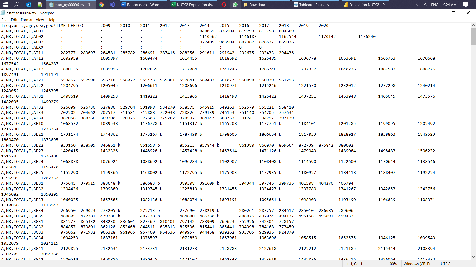
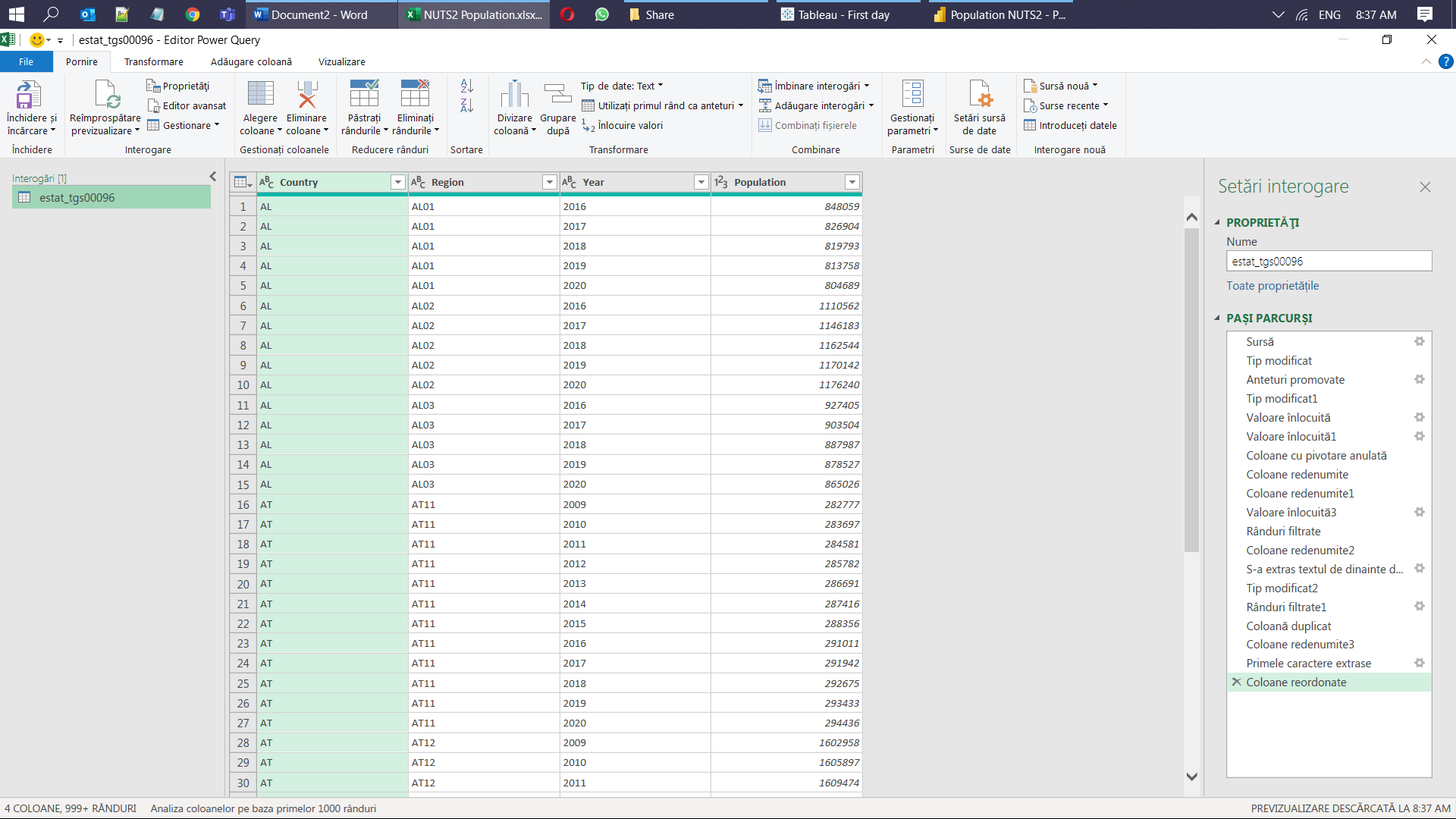
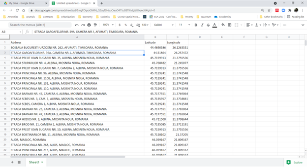
Data acquisition. Familiarization with the most important European and national level official data providers. For the European level the Eurostat website: https://ec.europa.eu/eurostat. Here we discussed the ways data is stored and it can be downloaded for analytical purpose. For the Serbian context, the Statistical Office of the Republic of Serbia: https://www.stat.gov.rs/en-US/. In the case of Hungary, we used the website of the Hungarian Central Statistical Office: https://www.ksh.hu/?lang=en. For Romania the main official data repository is the website of the National Institute of Statistics: http://statistici.insse.ro:8077/tempo-online/#/pages/tables/insse-table. Other important data sources for Romania are https://data.gov.ro/ that contains data sets from different national and regional level institutions or https://citadini.ro/ with city level relevant data related to the national urban policy. We have downloaded from Eurostat the European population at regional level in a tab delimited format (estat_tgs00096.tsv). We have vizualised in a text editor the data set: estat_tgs00096.tsv.
Data preparation in Power Query. We choose regional and country level population data in time series (from 2009 until 2020) for the European countries. The students learned to clean the data for all the unwanted fields and for missing data using the Power Query editor accessible both from Microsoft Excel and from Power BI. We transformed the data in a “normalized formed” to have the years as variables and all missing data was excluded. Also the name of the regions were standardized and a new column was created with the country codes. We have exported the edited data in comma separated values format.
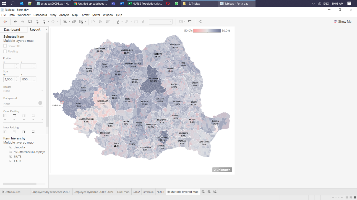
Session 4: Data visualization in Tableau
Teaching method: lecture and workshop
Duration: 120 min
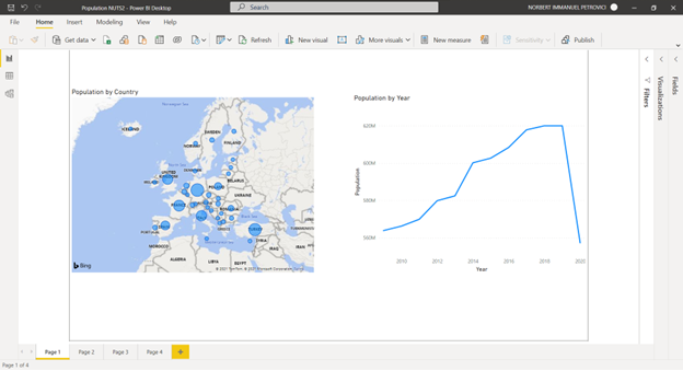
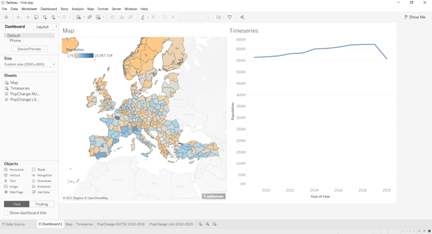
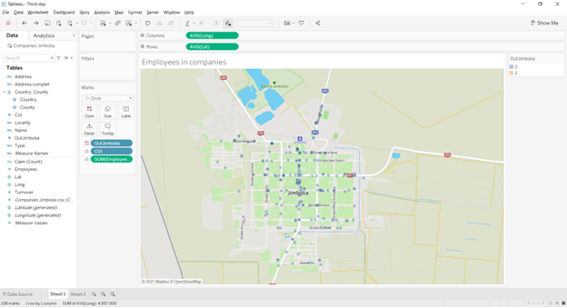
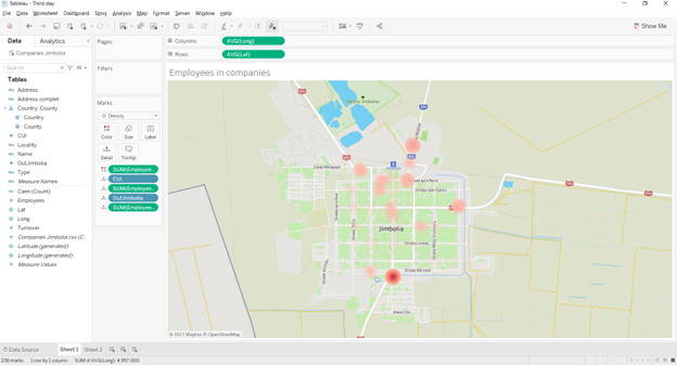
Content: We use Tableau from Saleforce to visualize the population at regional level and its aggregate dynamic. Also, the students are taught to create basic and complex charts. They are also introduced to maps and dashbords.
Session 5: Data Silos in Tableau
Teaching method: lecture and workshop
Duration: 120 min
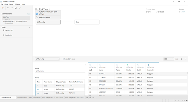
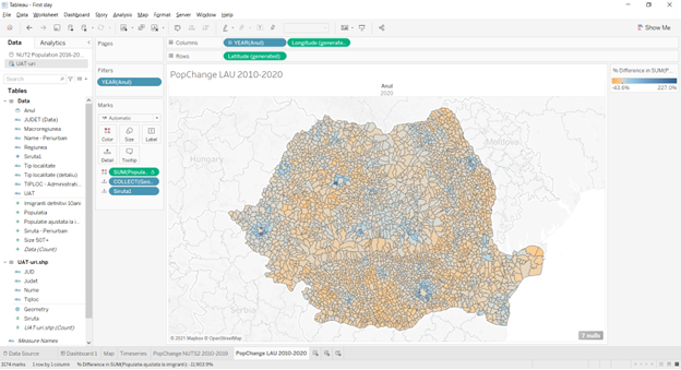
Content: The data silos concept was introduced and then the concept of relation between table of data. To exemplify, we load the locality level geographical file (in shape format) and relate it with the aid of a key with the dynamic of population data. We used the Romanian geo and the population files.
Session 7: The use of descriptive statistic in data visualization
Teaching method: lecture and workshop
Duration: 150 min
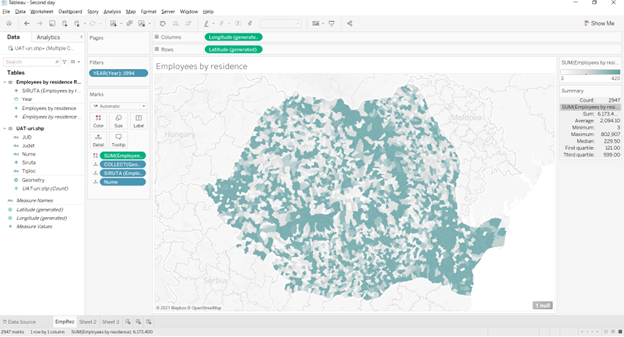
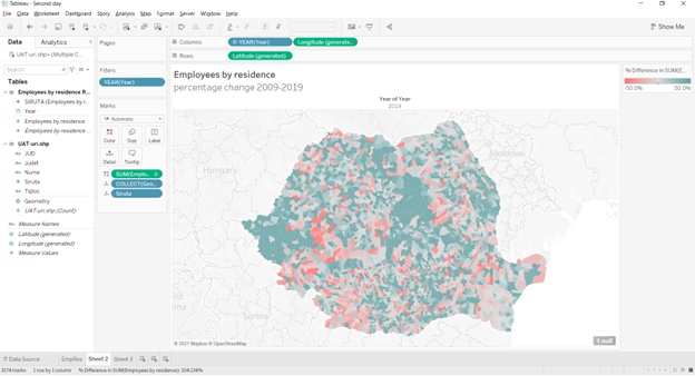
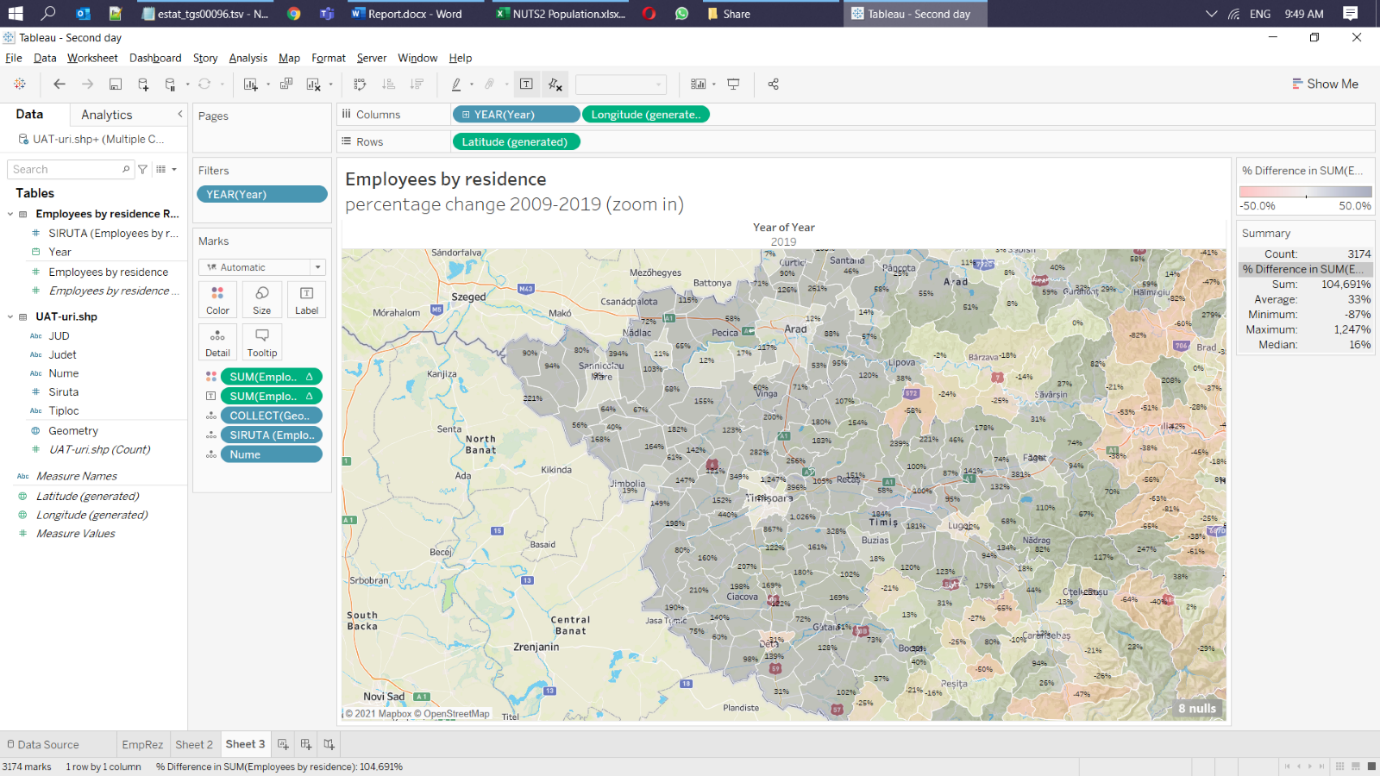
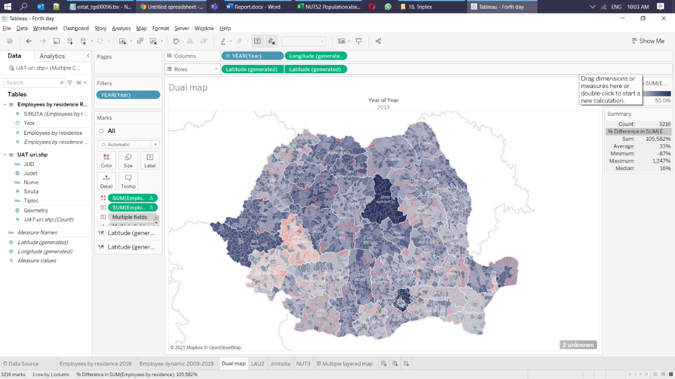
Content: We learn how to use descriptive statistics: mean, median and dispersion to centre and truncate the data in a visualization to grasp visually the major trends. We used the number of employees in Romania by their residence.
References
- Oprea D., Mesnita G., Dumitriu F. (2005) – Analiza sistemelor informaționale
- BABOK V3 (2019) – A guide to the business analysis body of knowlege – International Institute of Business Analysis
- Fotache M. (2009) – SQL. Dialecte DB2, Oracle, PostgreSQL si SQL Server: Polirom.
- Velicanu M., Matei G. (2010) – Tehnologia Inteligenta Afacerii: Editura ASE
- Muntean M., Bologa A.R. (2015) – Business Intelligence. Teorie și practică: Editura ASE
- Kimball R., Ross A. (2013) – The Data Warehouse Toolkit, 3rd Edition: Wiley
- AXELOS (2019) – An introduction to PRINCE2: Managing and Directing Successful Projects: TSO
- Sood A., Sinha N., Dewjee S., Zhao W. (2020) – Tableau Tutorial. User Documentation
- QlikTech International AB – Concepts in Qlik Sense
Other Instructors

Florin FAJE
Lecturer

Cristian POP
Lecturer

Norbert PETROVICI
Associate Professor

Anca CHIȘ
Communication specialist

Ionuț FÖLDES
Lecturer
Syllabus
The aim of this class is to understand in which categories do the cities from Romania fall from the perspective of the economic and social changes through which they underwent in the last decade? Does this typology indicate a change in the patterns of economic and social geography of Romania? Can we delignate the trajectory of specific cities in the new economic and social landscape? Take the case of Jimbolia: where does it stand? Is Jimbolia a growing, static or a shrinking city? What kind of resources and capabilities does it uses in the changing landscape of capital investments? The workshops will help students familiarize with the important steps in data visualization: data aquisition, data preparation (cleaning), the constructions of charts, data silos, using descriptive statistics, geocoding and the construction of complex maps. Tools used: Excel, Power Query, Power BI and Tableau.
O1.M2 OBJECTIVE AND SUBJECTIVE SKILLS IN INTERPRETING TERITORIAL NETWORKS
O1.M2.01 Tools for visualizing the urban geography of economic growth Case study: The urban geography of economic and social growth in Romania 2010-2020
Type of format
Lecture & Workshop
Duration
Session 1 – 120 min: The urban geography of economic and social growth in Romania 2010-2020 50 min lecture on theoretical notions related to the urban geography of economic and social growth 10 min break 60 min lecture on major cities typology Session 2 – 120 min: Data acquisition and data preparation 30 min lecture on data acquisition 20 min workshop on data acquisition 10 min break 20 min lecture on data preparation with Power Query 40 min workshop data preparation with Power Query Session 3 – 120 min: Data visualization in Power BI 10 min introductory lecture about Power BI 50 min workshop on constructing univariate charts with Power BI 10 min break 60 min workshop on constructing multivariate charts with Power BI Session 4 – 120 min: Data visualization in Tableau 10 min introductory lecture about Tableau 50 min workshop on constructing basic charts with Tableau 10 min break 60 min workshop on constructing complex charts with Tableau Session 5 – 120 min: Data Silos in Tableau 20 min lecture about data silos with Tableau 40 min workshop on working with data silos 10 min break 50 min workshop on working with data silos Session 6 – 80 min: Population dynamic charts 20 min lecture on population dynamic 60 min workshop on representing population dynamic in Tableau. Session 7 – 150 min: The use of descriptive statistic in data visualization 30 min lecture on the use of descriptive statistics in data visualization 50 min workshop on descriptive statistics in Tableau 10 min break 30 min workshop on data standardization 30 min workshop on data interpretation Session 8 – 120 min: How to geocode 10 min lecture on geocoding with Google services 50 min workshop on point representation of geographical data 10 min break 50 min workshop on density maps Session 9 – 120 min: Maps with layers 50 min workshop on constructing maps with two layers 10 min break 60 min workshop on constructing maps with multiple layers
Possible connections (with other schools / presented topics)
UAUIM O1.UAUIM01 / Grid and border as instruments of planning and criticism in architecture O1 M2. 03. Process vs Object. Working with post industrial communities SUSKO O1.SUSKO / Geographical tools in Territorial Exploration
Main purpose & objectives
The main purpose of this class is to help students to ask some of the important socio-economic questions about the urban geography of different cities. The objective is to help students understand the data visualizations steps and procedures. Also, the hands-on approach will help them use several contemporary data visualization tools.
Skills acquired
Detailed theoretical knowledge on urban geography and its relation with socio-economic phenomenon The ability to work with (spatial) data. All the steps implied in preparing the data, basic analytical skills and deep visualization abilities. Hard skills in working with several tools (i.e Power BI, Power Query, Tableau).
Contents and teaching methods
All of the above mentioned sessions will be based on a dynamic combination of lectures with a hands on approach in the several workshops for each topic.
Reviews
Lorem Ipsn gravida nibh vel velit auctor aliquet. Aenean sollicitudin, lorem quis bibendum auci elit consequat ipsutis sem nibh id elit. Duis sed odio sit amet nibh vulputate cursus a sit amet mauris. Morbi accumsan ipsum velit. Nam nec tellus a odio tincidunt auctor a ornare odio. Sed non mauris vitae erat consequat auctor eu in elit.
Members
Lorem Ipsn gravida nibh vel velit auctor aliquet. Aenean sollicitudin, lorem quis bibendum auci elit consequat ipsutis sem nibh id elit. Duis sed odio sit amet nibh vulputate cursus a sit amet mauris. Morbi accumsan ipsum velit. Nam nec tellus a odio tincidunt auctor a ornare odio. Sed non mauris vitae erat consequat auctor eu in elit.